Artificial Neural Network (ANN)

Artificial neural networks (ANNs) are types of computer architecture inspired by biological neural networks (Nervous systems of the brain) and are used to approximate functions that can depend on a large number of inputs and are generally unknown. Artificial neural networks are presented as systems of interconnected “neurons” which can compute values from inputs and are capable of machine learning as well as pattern recognition due their adaptive natureAn artificial neural network operates by creating connections between many different processing elements each corresponding to a single neuron in a biological brain.Implemented on a single computer, an artificial neural network is normally slower than more traditional solutions of algorithms. The ANN’s parallel nature allows it to be built using multiple processors giving it a great speed advantage at very little development cost.

The difference between neural networks and deep learning lies in the depth of the model. Deep learning is a phrase used for complex neural networks.

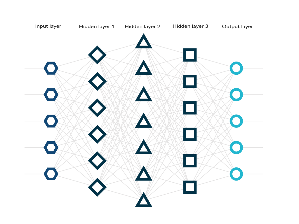
**Layers :**Input Layer : accepts inputsHidden Layer : set of linear models created with the first layerOutput Layer : linear models get combined to form a non-linear model

Perceptron vs Gradient DescentIn GD we take the weights and change them by Wi to Wi + a(y-y)xi [y can be any number between 0 &1]In Perceptron, not every point changes weights, only the misclassified ones. [y` can take 0 or 1 only]

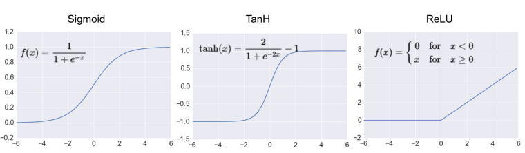
Activation Function :
In order to use 0/1 variables for classification, the gradient descent algorithm needs the error to be continuous and not discrete. In case the values are discrete, an activation function is used.The activation function converts the discrete step function (0/1) to a continuous function.
Sigmoid Function converts the numbers to a 0-1 scale with values closer to 1 for large positive numbers,values closer to 0 for large negative numbers and values close to 0.5 for numbers close to 0Softmax Function is the equivalent of the sigmoid activation function, but when the problem has 3 or more classes (outcomes).The softmax function requires all psigma(x) = 1 / (1 + exp(-x))Hyperbolic Tangent Function : Similar to sigmoid, but range between -1 to 1.Rectified Linear Unit (ReLU) : Simple function. If positive then same value is returned, if negative then returns 0.

Maximum Likelihood
Cross Entropy: If we have a bunch of events and a bunch of probabilities, how likely is it that those events happen based on the probabilities.If it’s very likely, then we have a small cross entropy. **Lower cross entropy is better.**If it’s unlikely, then we have a large cross entropy.
Sum of the negatives of the logarithms of the probabilities of the points. :: -ln(probability)
The likelihood or probability of an event is inversely proportional to the cross entropy.

**Error Function (Loss Function) :**Gradient Descent Algorithm (log-loss error)The error function should be differentiableThe error function should be continuousMean Squared Error

Feed Forward :
Epoch : One epoch is when an entire dataset is passed both forward and backward through the neural network only once
**Backpropagation :**In a nutshell, backpropagation will consist of:Doing a feedforward operation.Comparing the output of the model with the desired output.Calculating the error.Running the feedforward operation backwards (backpropagation) to spread the error to each of the weights.Use this to update the weights, and get a better model.Continue this until we have a model that is good.

Training :
Early Stopping : Keep doing Gradient Descent until the testing error stops decreasing and starts to increase. At that point we stop.Regularization : Large coefficients = Overfitting // Penalize large weightsL1 : Add sums of the absolute values of the weights, times lambda *( vectors with sparse weights :: good for feature selection)*L2 : Add the sum of the squares of the weights, times lambda. *(vectors with homogeneous weights :: better for training models)*Lambda = constant which tell how much to penalize the coefficientsDropout : Hold out nodes and feed-forward and back-propagate one epoch. Probability that each node will be droppedRandom Restarts : To avoid Local Minimas, which prevent the Gradient Descent from arriving at the bottom (global minimum), the Gradient Descent algorithm is started from a few places randomlyLearning Rate : How but steps are taken in order to reach the global minima. Higher rates are faster but inaccurate and may miss the minima and keep going.Momentum : Is the weight given to each step with the last step given higher weightage. This is done to avoid getting stuck at a local minima by jumping over with the average momentum. B is between 0 to 1.

L2 is better than L1. Example:PointsL1L2****Inference(0,1) 0 + 1 = 102 + 12 = 1L1 and L2 are both 1 in this case and are similar.(0.5, 0.5)0.5 + 0.5 = 1 0.52 + 0.52 = 0.5L1 is 1; L2 is 0.5. L2 has less error. Hence L2 preferred

Algorithm:We are at the top of the error and require a bunch of steps to reduce the error. This is done by Gradient Descent by going down in small steps following the negative of the gradient of the height, which is the error function.Each step is called an epoch.In each epoch, we take out input (data) and run it through the entire neural networkFind predictions and calculate the errorBack propagate the errors in order to update the weights in the neural network.

If we have many, many data points, which is normally the case, then these are huge matrix computations, I’d use tons and tons of memory and all that just for a single step.If we had to do many steps, you can imagine how this would take a long time and lots of computing power.Is there anything we can do to expedite this? Well, here’s a question: do we need to plug in all our data every time we take a step?If the data is well distributed, it’s almost like a small subset of it would give us a pretty good idea of what the gradient would be. Maybe it’s not the best estimate for the gradient but it’s quick, and since we’re iterating, it may be a good idea.This is where stochastic gradient descent comes into play. The idea behind stochastic gradient descent is simply that we take small subsets of data, run them through the neural network, calculate the gradient of the error function based on those points and then move one step in that direction.

Activation function: relu and sigmoidLoss function: categorical_crossentropy, mean_squared_errorOptimizer: rmsprop, adam, ada

DisadvantagesComputationally intensiveTends to overfit most times.